Dimension Tables – An Introduction

A Dimension table is one of the 3 key elements of dimensional modelling used to build a Data Warehouse. This article will give you an in-depth understanding of various Dimension table concepts.

What is a Dimension Table?

Conceptually, Dimension tables are database tables modelled to represent the business entities involved in business processes and events. The business processes are, in turn, modelled as Fact tables, and the Fact and Dimension tables are related in a “Star Schema” to provide an easy-to-navigate and query Data Warehouse database.

Where Fact tables represent the “numbers” you want to analyze, Dimension Tables provide the context by which you analyze those numbers. The Who, What, Where, When and Why.

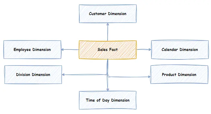
For example, imagine a typical Sales scenario. Employees sell Products to Customers. The Sales organization is divided into Divisions. Each Sale is a business event and, therefore, can be modelled as a “Sales” Fact. The diagram below depicts the Sales Fact and its related Dimensions. The Dimensions provide the Who (Customer, Employee), the where (Division) and the when (Calendar, Time of Day) context for the Sales Fact.

Dimension tables physically contain the descriptive attributes of the business entities. For example, a Customer Dimension would contain attributes like Customer Name, Age, and Gender. The attributes filter and group the Fact table data in reports and analysis. See the next section for more details.

How to Design a Dimension Table

A Dimension contains Members. There is a Member for every business/natural key of the Dimension. For example, in a Customer dimension, there is one member for each individual Customer. However, because a Dimension may keep the history of change for each member, there may be multiple rows in the Dimension table for each member, one for each version. To handle this, Kimball introduced the concept of a surrogate key.

Dimension Surrogate Key vs Business Key

Because a Dimension can keep multiple rows for different versions of any Member, the business key of a Member can be duplicated over multiple rows. Therefore, the business key can’t be used as the unique primary key. Instead, each row is assigned a unique surrogate key by the data warehouse. The surrogate key becomes the primary/unique key of the Dimension. Usually, a surrogate key is a sequentially assigned integer. In recent years generating a hash on the business key and effective date combination has become popular. There are cases where you may want to use a “smart” surrogate key. I.e. a code for the surrogate key. A typical example is the Calendar Dimension, with a smart key like “YYYYMMDD” used as the surrogate key for each row (representing a day) in the Calendar. Read more about Smart Keys.

Note that a surrogate key is only strictly needed for Dimension Tables, which contain type 2 (version history) attributes. However, I recommend assigning a surrogate key to every Dimension for uniformity and future-proofing.

Dimension Table Attributes

Attributes are the columns of Dimensions that contain descriptive information for each Member. E.g. Customer Name, Customer Income Level, Marital Status etc.

It’s important to understand that attribute values (not the attribute column names) become row and column headers in pivot tables/charts. For example, a pivot table showing sales by gender in the past 12 months would look something like this:

Where “female” and “male” are the values stored in the Gender attribute column of the Customer Dimension.

A mistake I often see is developers using codes or keys for values in attributes. So, for example, in the database, “male” and “female” are represented as the codes M and F. If the M and F codes are carried through to the Dimension Table, then the pivot table report looks like this:

Which is far less useful. Users looking at this report may have no idea what M and F stand for. The codes M and F should be converted to their meaningful descriptive values.

Some rules for Dimension attributes:

• Operational codes (e.g. M for Male, F for Female) should be converted in Dimensions to their descriptive format (i.e. Male/Female). 
• True/False, Yes/No values should be converted to descriptions like “Is Contractor” or “Is Not Contractor.”

Some red flags to watch out for:

• Dimension attributes should never be dates. Leave that to slowly changing dimension techniques, Calendar dimensions and various fact types.
• Numerical values, especially contiguous values, should not be used as Attributes. See the next section.

Discrete vs Contiguous Dimension Attribute Values

Dimension Table attributes should be discrete values, not contiguous values. What does this mean? Discrete values are drawn from a small set of distinct values, whereas continuous values can be any value (up to an infinite number) within a generally large range of possible values. A common example of a contiguous value that is often mistakenly used as a Dimension attribute is Product Price. For any given range of products a company sells, the product price could be any price between a range of say $0.01 and $10000.00. Its unlikely that any two products have the same price, which makes using price as a row or column header in a report not very useful. You will get a column or row for every price. See the example below. There is very little analytical value to a report like this:

To deal with this problem, a developer can turn the contiguous values into discrete values by defining groups of contiguous values. For example, a business might be interested in its sales of low-priced (<=$99), medium-priced (>$99 to <$200), and high-priced (>=$200) Products. By defining an attribute with values for each price range, the sales amount for each range can be aggregated and displayed. This is far more useful. See the image below:

Row Management Columns

A Dimension will also contain a set of “management” columns. Management columns are generally used by the ETL (extract, transform, load) process to help load data into the Dimension Table and to set properties of each row like latest flag, effective dates, etc.

Slowly Changing Dimensions (SCD)

Dimensions are often referred to as ‘Slowly Changing Dimensions’. The term recognizes that Dimension Members are relatively static but change (albeit slowly) over time.

This is important because users are often interested in the impact to their reports of these changes to Dimensions over time. It’s necessary to define a number of change-handling strategies for Dimension Table attributes. Ralph Kimball defined these change-handling strategies as Slowly changing Dimension (SCD) types 1, 2, 3 and 4:

• SCD Type 1 – Don’t keep history, i.e. overwrite.
• SCD Type 2 – Keep a version of the Dimension Member for every change.
• SCD Type 3 – Keep the latest version and the prior version (but not every version).
• SCD Type 4 – A hybrid combination of Type 2 and 3.

The most commonly used SCD strategies are Types 1 and 2. SCD Types 3 and 4 are rarely used.

An important nuance to note is that, although we talk about Slowly Changing “Dimensions”, what we are actually implementing is Slowly Changing Attributes. You implement the change-handling strategy per Attribute. That means different attributes within one Dimension can have different “slowly changing Dimension” types. There are various techniques to achieve this. The short answer is to use one hash management column for columns of type 1 and a second hash for columns of type 2.

Read a more in-depth description of Slowly Changing Dimensions, including example code you can download and test for yourself.

Slowly Changing Dimension Type 1 – Overwrite

The slowly changing Dimension (SCD) type 1 change-handling strategy is applied, if a change occurs to an attribute, the existing attribute value is overwritten with the new value. Essentially no history of the change is recorded.

A good candidate for an SCD Type 1 Attribute is something like Employee Name. If an employee’s name changes due to marriage, you don’t want two versions of the employee, one before marriage and one after. If you did and were looking at sales by employee, the employee would show up twice, once with the new name and once with the old. Instead, you want to overwrite the old name with the new name. In this scenario, the sales report by Employee would only show the Employee with the new name. Effectively all historical sales for that employee are now associated with the new name.

This highlights unanticipated consequences with SCD Type 1, and why you might want to adopt a different strategy (i.e. SCD Type 2). Let’s say you have a Sales Division Dimension, and each Sales Division has a parent Region. If the Sales Division is moved to a new Region, and the Region attribute of the Sales Division is treated as SCD Type 1, and overwritten with the new Region, then all the historical sales facts that were associated with the old Region would suddenly appear in Regional reports as if they had occurred in the new Region. Usually, an undesirable outcome. This is where SCD Type 2 comes into play.

Slowly Changing Dimension Type 2 – Add a new Version

In the SCD type 2 scenario, a new version of the Dimension member row is written when an SCD Type 2 Attribute changes. History is preserved. Existing Facts remain associated with the old version of the Dimension Member, and new Fact data is associated with the new version of the Dimension Member. For Example, let’s say you have a Sales Division Dimension, and each Sales Division has a parent Region attribute. A decision is made to move the Sales Division into a new Region. If the Region attribute of the Sales Division is treated as SCD type 2, then a new row is written to the Dimension Table for the new version of the Sales Division Dimension Member. There are now 2 rows in the Dimension for the same Division, one with the old Region, and one with the new Region.

All the existing Sales facts associated with the old version remain associated with that version and would still appear in Regional reports as if they belong to the old Region. This is a desirable outcome because this region was responsible for each Sale at the time it was made. Only new Sales that occur after the change are associated with the Sales Division with the new Region, thus preserving history.

Slowly Changing Dimension Type 3 – Latest and Prior Version

SCD Type 3 change-handling strategy captures the latest and prior value of a Dimension attribute. It doesn’t capture every version. There are some rare circumstances where this is desirable. Take the previous example of a Division moving Regions. What if the business wanted to see today’s sales “as if” they were in the old region just to compare how they would have performed under the old sales organization? The SCD Type 2 strategy doesn’t accommodate this kind of request. This is because new sales are never associated with the old region. For a period of time, they may want to track sales in terms of the old regional divide vs the new regional divide.

Type three SCD satisfies this kind of reporting requirement. In the SCD Type 3 strategy, you don’t create a new row for the version of the Dimension member. Instead, a new column is added to capture the prior value.

For example:

Before the change the Richmond Division is in the “North” East Region:

A “prior region” column is added to the table to accommodate the SCD type 3 change, and then the Richmond Division is moved to the “East Coast” Region. The result is as follows:

Now all Sales Facts, new and old, are associated with the single version of the Dimension member, but analysts can choose either the current Region or Prior Region (or both) in their reports to compare current to prior Regional organization sales.

Dimension Table Denormalization vs Normalization

Dimensions often represent hierarchical relationships in the business. For example, take a Division->Region->Country hierarchy. In an operational system, these would normally be modelled as separate (normalized) tables with relationships between them. However, Dimensions tend to be denormalized. That is, instead of separate Dimension tables, we would have a single Division Dimension. The Division Dimension has a Region and Country attribute to model the relationship between a Division and its Region/Country. The hierarchical descriptive information is stored redundantly, but this design results in improved ease of use and query performance. Dimensions tend to have relatively few rows compared to Fact tables and a large number of columns. The trade-off with storage space is insignificant.

The exception would be if there were Facts in the Data Warehouse that had a grain at the Region or Country levels; then it’s necessary to have separate Dimensions for those levels so those Facts can be attached at that level.

Snowflake Dimensions

Snowflake dimensions describe hierarchical relationships in a Dimension table that have been “normalized.” Instead of a single Dimension Table with attributes representing relationships, secondary Dimension tables are created and connected to a base Dimension by an attribute key.

My advice (and Ralph Kimball’s) is to avoid them. They simply make the Data Warehouse harder to navigate, and nothing can be modelled in a Snowflake schema that can’t be modelled in a Star Schema.

Read Snowflake vs Star Schema for more information

The Two Types of Dimension Hierarchies

Natural Hierarchies

Many dimensions contain natural relationships between attributes that form hierarchies. In our previous example, in the Division Dimension, there is a hierarchy from Country->Region->Division. This is known as a “natural” hierarchy because it is a relationship between attributes with a fixed depth or number of levels.

Hierarchies can be very useful for analysis, allowing drill-down and drill-up analysis in BI tools. BI tools can be configured to show these hierarchies as nested attributes making it easy to visualize and navigate the hierarchy.

It’s common for Dimensions to have multiple hierarchies. For example, a Calendar Dimension can have a Day>Month>Year… a Day>Month>Fiscal Year… a Day>Month>Quarter>Year and a Day>Fortnight>Year hierarchies. All are valid Hierarchies, and all may be used by different people for different purposes.

Some Natural Hierarchy rules:

• Hierarchies in a Dimension always end with the root Attribute at the Grain of the Dimension. E.g. In the Calendar Dimension, the Day Attribute.
• It’s important that each attribute value belongs to only one of its parent Attribute values. Otherwise, you have a broken Hierarchy.

Parent-Child Hierarchies

A Parent-Child Hierarchy is a hierarchy of Dimension members where child members “point to” their parent members. Parent-child hierarchies are also known as Ragged or variable-depth Hierarchies because each “branch” of the Parent-Child “tree” can have a different number of levels.

Employees or Positions in an Organisation Chart are good examples of parent-child hierarchies. Each object points to its parent object, i.e., each Position in an Organisation Chart points to its parent Position.

These kinds of relationships are known as “recursive” relationships. Recursive relationships have traditionally been difficult for SQL and BI tools to navigate. Thankfully, today, most SQL dialects and good BI tools can natively query these relationships or emulate natural hierarchies based on the parent-child hierarchy.

Some Parent-Child Hierarchy rules:

• A Parent can have multiple children, but a child only has one parent.
• The child contains an attribute that contains the identifier of its parent.

The Importance of Conformed Dimensions

The Kimball method of Data Warehouse design describes a Data Warehouse Bus Matrix Architecture and the concept of “conformed” dimensions. Put simply, the concept of “conformed” Dimensions states that Facts should share common or “conformed” Dimensions to enable cross Datamart/Enterprise/Business process analysis.

The aim is to design your data warehouse so that Facts share as many Dimensions as possible. A data warehouse bus matrix is a good way to document the design of your Data Warehouse and maximize conformed Dimensions.

A Data Warehouse matrix documents the relationship between all planned Facts and Dimension Tables. By completing a matrix, you can see the overall high-level design of your Data Warehouse on a single sheet. In the image below, where there is a “1” at the intersection between Facts (the rows in blue) and Dimensions (the columns in green), there is a relationship between the Fact and the Dimension.

Conformed Dimensions are powerful. They allow cross-fact analysis. If two Facts share a Dimension, then, when a member is selected in that Dimension Table in a BI tool, it filters both Facts. For example, let’s say you have sales and accounting fact tables that are connected to the same calendar dimensions. You can select a Calendar period (e.g. Month), and select measures from both Fact tables (e.g. Sales Qty, and Revenue) in the same pivot table and they are both filtered by the Calendar Period member. See below:

This also allows you to define calculated measures that use measures from more than one Fact table. For example, the “Avg Sale Amount” above which is Revenue/Sales Qty.

Role Play and Junk Dimensions

Role Play Dimension

A Fact can be associated with a Dimension in a different role more than once. These secondary associations are known as Role Play Dimensions. For example, a Task fact can be associated with the Calendar Dimension a number of times: once for a Scheduled date, once for a Started date, once for a Completed date and so on. Each of these would appear as separate Dimensions, i.e. the Started Calendar Dimension, the Scheduled Calendar Dimension and the Completed Calendar Dimension. This structure allows you to use the Scheduled Calendar, for example, to get the count of Tasks scheduled to start in a month. You could use both the Schedule and Started Calendars to get a count of Tasks that were both Scheduled and Started in a month. If you are directly querying your relational Data Warehouse, it’s useful to create a view for each role-play of the calendar. If you are using OLAP, it is not necessary.

Junk Dimensions

Transactions typically produce a set of miscellaneous, low-cardinality flags and indicators associated directly with the transaction. E.g. Sale Type, Sale Status etc. Our first instinct is to create a Sale Dimension to “house” these flags and indicators. However, a Sale Dimension would have one member for every Sale. That would mean the Dimension Table potentially has millions, hundreds of millions of rows, or even billions of rows. This would result in very poor performance.

Another remedy is to create a separate Dimension for each flag or indicator. However, this leads to a proliferation of Dimensions.

Rather than making separate dimensions for each flag, the best remedy is to combine them in a single “Junk” or degenerate dimension. Junk dimensions contain either the full Cartesian product of all attributes’ possible values or a combination of just the values that actually occur in combination within the source data.

Using the cartesian product is generally less resource-intensive. To generate a list of only existing combinations means scanning the whole source transaction table.

The more attributes you have in the Dimension, the bigger it gets. It’s important that the attributes are low cardinality. If you have 10 * 345 * 81 * 3 * 21 attribute values, you have 17M+ members. So you need to be careful what you include. In this case, perhaps the attribute with 345 values can be separated into its own dimension.

The business key of Junk Dimension is the combination of all attributes. When you do a lookup from the Fact to the Dimension to associate the correct member of the Junk Dimension, you need to combine all the attributes as the Lookup value. One tactic is to create a single business key column with a concatenation of the attribute values or a hash of the attribute values.