Data Warehouse Architecture

What is Data Warehouse Architecture

Before you build a data warehouse, you must define some standards for how you and your team will design and structure your data warehouse system. A Data Warehouse Architecture describes how data is sourced, stored, processed, and accessed. The architecture can vary depending on the specific needs and scale of the organization, but generally, it will follow a layered approach.

There have been various Data Warehouse Architecture articulated by well-known experts in the field. These architectures have included:

• Kimball Dimensional Data Warehouse Architecture
• Inmon Data Warehouse Architecture
• Data Lakehouse Architecture
• Data Vault Architecture

What all these architectures have in common is they are layered, include a dimensional presentation layer and exhibit the characteristics outlined below:

1. Integrated. A data warehouse takes a copy of the data (on a regular basis) from the enterprise’s application systems. It integrates that data into “one place”, simplifying data access for reporting purposes. A second form of integration is to match and merge data from multiple systems into single subject-oriented entities.
2. Subject-oriented, not source system-oriented. A data warehouse reorganises the source data into business subjects/domains, making it easier for users to understand and consume.
3. Historical/Time Variant. A Data Warehouse records the history of how data changes. This is important for accurate reporting, auditing and efficient data management.
4. Non-Volatile. Data is loaded in periodic “batches”. The data doesn’t change from moment to moment; rather, it’s stable between load periods. This means reporting and analysis can be conducted without the data changing underneath you.

Here, you will discover the latest thinking in modern data warehouse design. It represents a blend of previous architectures, selectively incorporating the best elements from established designs.

Modern Data Warehouse Architecture

The modern Data Warehouse architecture has evolved to meet the growing demands of big data and data science, leveraging new technologies to do so. It selectively integrates the most effective elements of traditional architectures, resulting in a mature, comprehensive platform that can address a wide range of use cases. The key factors driving this evolution include:

• New “big data” technologies like Hadoop and Spark (e.g. Databricks).
• A desire to unify data warehousing and business intelligence with new requirements like machine learning, data science, and reverse ETL.
• The advent of Cloud data platforms (like Databricks, Snowflake and Fabric).
• Many years of experience of leading practitioners.

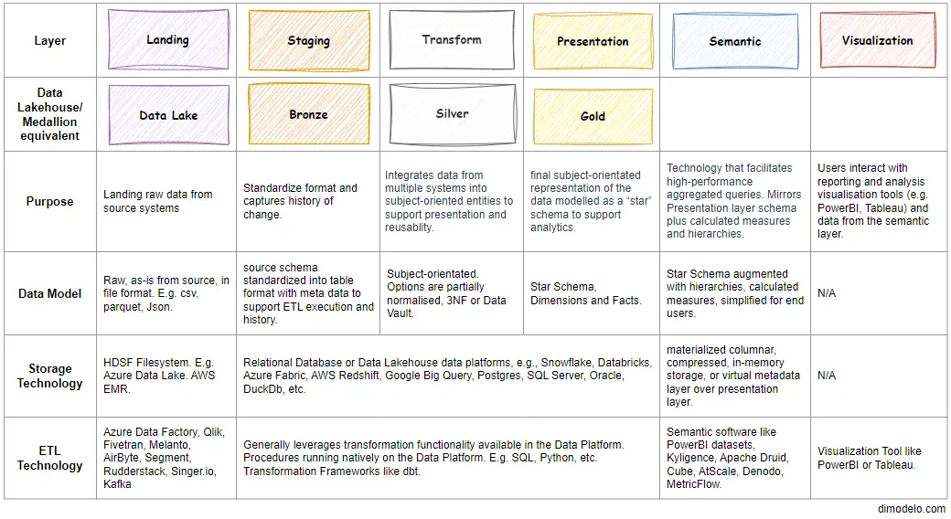
The modern data warehouse architecture consists of 6 Layers, including the Visualization layer. The diagram below summarizes each layer and its purpose and contrasts it with the Data Lakehouse architecture.

This may seem unnecessarily complex, but the layered approach simplifies the architecture technically and conceptually, with each layer serving its role and purpose. The design principles behind this layered approach are well-known software engineering principles that have matured as software design and delivery have matured. They include:

• DRY (Don’t Repeat Yourself): Avoid redundancy by ensuring that every piece of logic is represented only once in the codebase.
• Separation of Concerns: Divide into components, each addressing a separate “concern” or doing a different “job” to simplify manageability and maintainability. The layered approach is an example of the separation of concerns.
• Patterns: Data engineers who work with data warehouses or lakehouses for an extended period will begin to identify recurring code patterns. They often repeat the same code over and over for multiple entities. Adopting a layered approach with a “separation of concerns” can help isolate these patterns, allowing for standardization and, eventually, automation.
• Portability: Data platforms change over time, and new platforms are arising at an ever-increasing pace. You don’t want to be locked into any one vendor. At Dimodelo, we emphasize defining architectures and patterns that can be implemented with any data platform, ETL tool, or transformation language. The tools can change, but the architecture, standards, and patterns remain the same.

A key aspect of the modern data warehouse is how data flows through each layer. The process of “moving” the data is known as ETL, an acronym for Extract, Transform and Load. The diagram below is an overview of the various processes that occur to load each of the layers. The layered approach allows for the separation of concerns at each layer. This, in turn, allows us to identify, implement and even automate common patterns and standards at each layer.

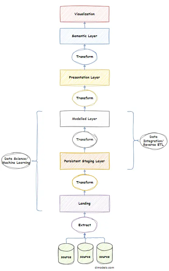
You’ll notice that the modern data warehouse architecture shows a relationship to Data Science/Machine Learning and Data Integration/Reverse ETL. I address these aspects in the “Extending the Data Warehouse Architecture” Section.

Layers of the Data Warehouse Architecture

Landing Layer

The sole function of the landing layer is to “land” or store the data retrieved from source systems, which is ready for further processing. In today’s world, this data can be in various formats, such as structured (tabular), semi-structured (e.g., XML, JSON), and unstructured (e.g., emails, documents). The Landing layer must be capable of capturing all of it. The Landing layer is the equivalent of the underlying data lake of a Data Lakehouse medallion architecture.

Typically, the Landing layer is implemented as a file system (such as HDFS or Data Lake) where an ETL Extraction tool deposits files representing data extracted from source systems. The ETL tool will read structured or semi-structured data in its raw format and write it in a standardised format (e.g., parquet, proprietary, CSV, etc.). This standardised format helps standardize and automate the downstream Staging layer ETL patterns.

The Landing layer data can be transient. That is, once a Persistent Staging Layer has captured the data, the data can be deleted. However, in some cases, especially for unstructured data, there may be good reason to keep the data in the Landing layer, typically for machine learning or data science purposes.

Landing layers are often loaded with dedicated Extraction tools like Airbyte, Fivetran or Qlik. These tools specialize in connecting to source systems, extracting data incrementally where possible, and landing it in the Landing layer. They typically excel at this job but don’t work well (if at all) at transforming the data.

The data schema in the Landing layer model will match the source systems schema.

Typically, the landing layer is only accessible to data engineers responsible for creating and maintaining it. The exception may be data scientists working with unstructured data.

Extract patterns tend to fall into one of the below:

• Full Extract. All the data in the source entity is extracted.
• Incremental Extract. Only the changed data is extracted from the source. This method is much faster than a Full extract. However, the source entity must support it. For the pattern to work, you need to identify a column or multiple columns that the source system uses to track change. They would usually be a modified date or sequential identifier. The downside of this pattern is that it doesn’t detect hard row deletes from the source. That makes it necessary to run a period Full Extract as well.
• Change Tracking. The change tracking pattern uses the change tracking mechanism of the source system(e.g., change tracking in Microsoft SQL Server) to identify changes in the source entity and extract only changed data. The Change Tracking pattern has an advantage over the Incremental pattern in that it recognizes hard deletes and is, therefore, a superior pattern if available.
• File Pattern. Extracting files is quite simple—it’s effectively a copy-and-paste. However, files can be very unreliable and variable in nature. There may be many files in the source that represent a single entity. The files might represent Full, Incremental, Change tracking or Date Range extracts. Files are probably the most unreliable with respect to their schema stability. From an extract perspective, file sources are reasonably simple but quite complex from an ingestion standpoint.
• Date Range Pattern. The date range pattern is used to extract a subset of the source data based on a date range. The end of the date range is the “current” date, and the start range is the number of days before the current date. The date range ‘window’ moves forward a day as the current batch effective date changes. For example, you might have a very large transaction table that doesn’t support either incremental or change tracking. Instead of doing a Full extract every day, you might only extract the last 31 days of transaction data each day to capture any changes that have occurred in the last month.

(Persistent) Staging Layer

Traditionally, the Staging layer served as a temporary area where raw data was collected, cleaned, and prepared before being transformed and loaded into the Presentation layer. In the modern data warehouse architecture, the Landing layer now assumes the role of data “collection”, while the Staging layer has evolved into a “persistent” Staging layer that permanently records the source data and its change history.

The Staging layer is the equivalent of the Bronze layer of the Data Lakehouse medallion architecture.

The Persistent Staging layer serves as a reliable foundation of the data warehouse. If all else fails (literally), the higher data warehouse layers can be rebuilt from this foundation. Indeed, as long as the Persistent Staging layer stays consistent, you can confidently change, modify and reload higher layers with full history without losing data. This wasn’t possible with older data architectures where the Presentation layer was the first persistent layer in the architecture. The concept of a Persistent Staging layer evolved because of problems with reloading and changing the Presentation layer, which resulted in historical data loss.

The schema of persistent staging data is tabular based, in either a database table format or file-based formats that lend themselves to tabular formats, such as Parquet with Delta table or Apache Iceberg.

The schema of the persistent staging layer closely mirrors the source system schema, except for some additional data management columns used for handling history and ETL processes. While the format might change, such as converting from JSON to tabular, resulting in some flattening, the column names and structure remain the same. There should be no data transformation.

Modern data platforms like Databricks, Snowflake, and Microsoft Fabric can directly read files from a Landing layer. The code required to write data and maintain history in a target persistent staging table can be implemented on your preferred data platform.

Typically, the ingestion pattern for Persistent Staging entities can be standardised.

• Identify the delta change data set, I.e., only the data that has changed since the last execution. This depends on the extract pattern used to extract the data from the source. Identifying the delta change set is easy for Incremental and Change Tracking patterns. A full comparison with the target persistent staging entity is required for Full extracts. A full comparison with the target Persistent Staging entity over the date range is required for date range extracts. For file extracts, it’s dependent on the pattern the file represents.
• Once identified, the delta change set can be applied to the target persistent staging entity in a straightforward and standardized way.

Modelled Layer

The “modelled” layer is also known as the “Core” or “Middle” or “Reconciled” or “Transformed” layer. We chose the word “Modelled” because it seems the most descriptive to us.

The Modelled layer marks the beginning of the data’s transition into a subject-oriented format. This layer is where the complex process of transformation takes place. Here, data from various systems is commonly consolidated and transformed into entities within a subject area. Data from multiple systems is matched and integrated to form a whole-of-enterprise view of key data entities. It serves as the central enterprise business model on which all enterprise reporting is built, not directly but as the foundation. The Modelled layer is the equivalent of the Silver layer in the Data Lakehouse medallion architecture.

The important thing is that the data model is subject-oriented. “Subject-oriented” refers to the organization of data around the key subjects and entities of the enterprise rather than around the source system representation (schema) of entities. Data is grouped by major subjects with entities relevant to that subject area, such as customers, products, sales, or orders. Each subject area is designed to provide a comprehensive view of the data related to that area.

Subject-oriented data modelling ensures that sometimes complex business logic is captured in one place, adhering to the DRY principle. This makes data consistent and standardized across the enterprise, reducing redundancy and discrepancies. Organizing data around subject areas fosters a common understanding across the enterprise and makes accessing data related to specific areas of interest easier for developers.

Remodelling your data from the source schema to your own subject area model decouples higher layers (i.e., presentation, semantic, and reporting) from source systems. If a source system is replaced (as it often is), it just requires “plugging in” the new source system to the existing Modelled layer schema. No reports, presentation, or semantic layer code must change (in theory).

The Modelled layer data model can take a few forms. Different teams and data architects have their preferences. The options include:

• 3rd Normal Form. 3rd normal form is highly normalized data usually used in the database of operational systems. It’s often overkill for the Modelled layer of a data warehouse, but it does provide norms and structures for developers to follow. Bill Inmon’s corporate information factory is an example of this approach.
• Data Vault. A Data Vault is designed for the modelled layer of a data warehouse. However, practitioners often find it difficult to understand and apply consistently. The criticism of data vault is its “explanation tax” where you “spend a lot of time explaining the nuances to stakeholders, both technical and non-technical”. I personally am not a fan. It’s a lot of work for little return.
• Pragmatic. A pragmatic approach simply treats the Modelled layer as a stepping stone to the presentation layer. It doesn’t follow any particular rule set or modelling technique. It’s usually highly denormalized. It can work for smaller teams where the primary outcome is business intelligence, reporting, and analytics. It requires the least effort but can become unruly after some time.
• Hybrid. A hybrid approach is a cross between the 3rd Normal Form and the Pragmatic. It still identifies key subject-oriented entities and their relationships but is pragmatic in allowing denormalization to support the presentation layer.

At Dimodelo, we favour a hybrid approach. The modelled layer must trade off effort and utility. We favour a third Normal Form schema, with denormalized tables wherever possible. Modelling is an art, not a science, so it’s difficult to define an exact description of how this is achieved. In later posts, I’ll develop some examples.

Modern data platforms such as Databricks, Snowflake, and Microsoft Fabric provide procedural languages like SQL and Python that you can use to implement the entities in the Modelled layer.

Presentation Layer

The presentation layer is the final subject-oriented representation of the data designed specifically to support business intelligence use cases such as reporting, ad hoc analysis, and dashboards. It is modelled using a strict Star Schema, which is comprised of Dimensions and Facts and their relationships. Data in the Modelled layer is read and transformed into the Dimensions and Facts of the Star Schema. The Presentation layer is the equivalent of the Gold Layer in the Data Lakehouse medallion architecture.

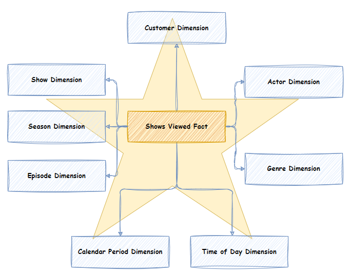
The Star schema is used because of these characteristics:

• The Star Schema is an easy-to-understand and navigate data model that supports multiple analytic use cases.
• Because of its simplified joins, a Star Schema supports high-performance aggregated queries. It performs well over many different analytics use cases.
• Star schemas are broadly accepted and used across the industry.
• The Star schema is the schema expected by Semantic layer tools. The semantic layer can consume Star Schemas as-is and apply various compression and pre-aggregation techniques to further enhance aggregated analytical query performance.

Because of the nature of the Star schema, it is easy to implement standardized patterns to load Facts and Dimensions. Check out our Slowly Changing Dimension article for an example.

Modern data platforms such as Databricks, Snowflake, and Microsoft Fabric provide procedural languages like SQL and Python that can be used to implement the entities in the Presentation layer.

Semantic Layer

The semantic layer is typically exposed to end users for business intelligence, ad-hoc analysis, reporting, and dashboard use cases. End users interact with the semantic layer via visualization tools like PowerBI or Tableau.

A semantic layer is implemented in a technology that facilitates high-performance aggregated queries over large amounts of data.

The semantic layer’s data model mirrors the presentation layer’s Star Schema. It further augments the data model with calculated measures and hierarchies that other technologies cannot create.

There are several styles of Semantic layers, including materialized, virtual or hybrid. There are also various tools and vendors. PowerBI implements a semantic layer. Other materialized/hybrid semantic layers include Kyligence, GoodData, Apache Druid and Apache Pinot. Some virtual/hybrid semantic layers include Cube, Malloy, LookML, Metriql, AtScale, MetricFlow, Metlo, and Denodo.

The Ralph Kimball approach to Data Warehouse architecture focuses on creating smaller data marts optimized for specific business areas with conformed dimensions unifying the data marts. Practically speaking, the value of a data mart is to present a subset of the data warehouse that only includes data relevant to a business area or user group. This can be achieved by developing multiple semantic models. The added advantage is the ability to apply security at the semantic model level.

Read a deep dive into semantic layers for further information.

Visualization Layer

The visualization layer of the data warehouse refers to the set of tools and technologies used to present and visualize the data stored within the presentation/semantic layer of the data warehouse. You deliver meaningful insights through various forms of visual representation, enabling users to understand trends, patterns, and relationships in the data. Components of the visualization layer typically include:

• Dashboards: Interactive, real-time interfaces displaying key metrics and performance indicators through charts, graphs, and gauges.
• Reports: Predefined and ad-hoc reports that present data in a structured format, often with tables, charts, and summaries.
• Data Visualization Tools: Software that allows users to self-serve, creating custom dashboards and reports.
• Ad hoc Analysis tools facilitate multidimensional analysis, often providing pivot tables and drill-down capabilities that enable users to explore data and generate insights.
• Business Intelligence Portal: Providing online access to reports and dashboards, organised in relevant folders, groups and departments. User and developers can publish their reports to the Portal, making them available for others to use. The portal provides safeguards like access control.

Examples of popular tools used in the visualization layer include Tableau, Power BI, Looker, and QlikView. These tools provide user-friendly interfaces that enable business users, analysts, and decision-makers to interact with and interpret the data effectively.

A Visualization layer won’t typically store data. It simply queries and presents the data from the presentation/semantic layers.

ETL/Data Integration

“ETL,” is an acronym for Extract, Transform, Load. It describes the process of extracting data out of one data store transforming it, and loading it into another.

Initially, data warehousing comprised only two layers: Staging and presentation. At the time, ETL referred to the process of extracting data from its origin, transforming it to fit the star schema, and then loading it into the Presentation Layer. Although the term ETL is still used today, it’s difficult to neatly apply the concept to the multiple layers of modern data warehouse architecture. In reality, every layer has some aspect of extract, transform and load. Nonetheless, the ETL terminology endures, and we continue to use it when describing the movement of data through the various layers.

Some people characterize ETL in modern data warehouses as data extracted from source systems, transformed into a Modelled layer, and then loaded into the Presentation layer. However, this description does not really depict the reality of the ETL system.

Instead, in the modern data warehouse architecture, I like to think of each Layer having its own mini ETL process:

• Landing Layer. Data is extracted from the source and loaded into the Landing data store.
• Staging Layer. Data is extracted (or, more precisely, queried) from the Landing layer, lightly transformed into tabular format (with history), and loaded into the Staging layer datastore.
• Modelled Layer. Data is extracted (or, more precisely, queried) from the Staging Layer, transformed into a subject-orientated and loaded into the Modelled layer data store.
• Presentation Layer. Data is extracted (or, more precisely, queried) from the Modelled Layer, transformed into a star schema, and loaded into the Modelled Layer data store.
• Semantic Layer. Data is simply loaded into a Materialized Semantic Layer. Data is not loaded into a Virtual Semantic Layer.

I think this description more accurately reflects the reality.

In the following sections, I’ll discuss Extract, Transform and Load in more detail.

Extract

As I’ve discussed, every layer of the modern data warehouse architecture has its own version of “extract”, but in this section, I want to focus on the process of extracting data from a source system and loading it into a Landing layer data store.

A core part of your technical Data Warehouse architecture will be the tool you use to implement data extraction from source systems. Generally, these tools specialize in extraction and exist in your architecture purely to fulfil that role (i.e. separation of concerns). All these tools should have these features:

• Ability to connect to a broad array of source systems and databases (usually in the hundreds).
• The capability to support either batch, data streaming, or both methods of extracting data. Batch is the most common method for Data Warehouses. It involves scheduled extraction of multiple rows of data (i.e., batches) in bulk. Batch extraction is reasonably straightforward and easily understood. Streaming involves continuous real-time or near real-time “streaming” of individual source system transactions. Streaming is more difficult to implement and maintain but may be necessary to support real-time analytics and reverse ETL use cases.
• Support a variety of extract patterns like Full, Incremental, Range and Change Tracking.
• Ability to load data into various target datastores (e.g. AWS S3, Azure Storage) in a standardised format (e.g. parquet, CSV, JSON).
• Support Scheduling, restart and recovery.
• Support workflow monitoring.

There are many dedicated Extraction tools. Some examples are Airbyte, Singer.io, Kafka, Fivetran or Qlik.

Transform

In the early days of Data Warehouses, there was only one “transformation” step from the Staging layer to the Presentation Layer. Today, there are multiple transforms, from Landing to Staging (a very light transformation), Staging to the Modelled Layer, and Modelled Layer to Persistent Layer.

Transformation is the code that is written and executed to transform the data from one layer’s schema/format to another. It typically includes a combination of:

• Matching entities across various source systems
• Merging data from multiple entities across multiple source systems into a single entity
• Joining data across entities
• Cleansing data, identifying and correcting errors, inconsistencies, and inaccuracies.
• Summarizing data at higher grains
• Denormalizing data into larger, consolidated tables, introducing redundancy to support simplified high-performance queries.
• Remodeling data into a subject-oriented schema.

Transformation is typically built within your core data platforms, such as Databricks, Snowflake, or Microsoft Fabric. These platforms provide procedural languages like SQL and Python that you can use to implement transformation logic. At Dimodelo, we recommend tools like “dbt,” which are platform-agnostic, provide data engineering automation, significantly reduce development time, and improve consistency.

Load

I confess that the L( i.e., Load)in ETL has often confused me. Isn’t it just a given that after you transform data, you load it into a data store? What’s the big deal? Well, it turns out that’s pretty much all there is to it!

Each layer in a modern data warehouse possesses its own “Load,” which results from a transformation process. Typically, the target is a single entity within a layer, usually a table in the Staging, Modelled and Presentation layers. Within the Landing layer, an entity is often implemented as a folder that receives all the extracted files corresponding to an entity from the source.

Loading a materialized Semantic layer is generally straightforward. The tool used to implement the Semantic layer will be able to load data, either incrementally or in full, directly from the Presentation Layer.

Data Warehouse Architecture Components

If you are going to implement a data warehouse, there are several technical/software components you need to consider:

• Landing Data Store: A temporary storage area where raw data is initially landed before processing; examples include Amazon S3 and Azure Data Lake.
• Data Extraction Tool: Software that pulls data from various source systems into the data warehouse. Some examples are Airbyte, Singer.io, Kafka, Fivetran or Qlik.
• Data Platform: The foundational infrastructure that processes and stores data within the data warehouse, often including databases and processing frameworks. The compute and storage within the Data Platform are often managed separately and can scale independently. Examples include Snowflake, Databricks, Google BigQuery, and Microsoft Fabric.
• Semantic Layer Tool: A tool that facilitates high-performance aggregated queries over large amounts of data; examples include AtScale and PowerBI.
• Business Intelligence Tool: Software that allows users to visualize and analyze data through reports and dashboards; examples include Tableau, Power BI, and Looker.
• Development:
  • Code Repository: A version-controlled storage space for source code and development artifacts, enabling collaborative development and change tracking; examples include GitHub, GitLab, Azure DevOps and Bitbucket.
  • Agile Management Tool: Software that supports Agile project management methodologies, facilitating sprint planning, tracking, and collaboration; examples include Jira, Trello, and Azure DevOps.
  • Data Warehouse Automation Tool: A tool that automates the transformation of data within the warehouse, enabling modular and maintainable data workflows; dbt (Data Build Tool) is an example.
• Scheduling and Monitoring Tool: Software that manages and monitors data workflows, ensuring that tasks are executed at the right time and in the right order and provides user monitoring of progress. Examples include Apache Airflow and dbt.
• Network, Security, and Access Control: Mechanisms and tools to ensure secure data transmission, protect data from unauthorized access, and manage user permissions; examples include AWS IAM, Azure Active Directory, and Okta.
• Reference Data Management: The process of managing data lists for analytics classification or mapping purposes. It can be as simple as storing .csv files or as complex as master data management systems like Ataccama.
• Data Quality Management and Reporting: Tools and processes to ensure that data meets quality standards, with capabilities for profiling, cleansing, and reporting.

Extending the Data Warehouse Architecture

Data science and Machine Learning

The number one complaint Data Scientists make is how much time they need to spend sourcing and transforming data to prepare it for input into their data science models. With the modern data warehouse architecture, it’s possible to unburden Data Scientists from the chore of sourcing data and instead allow them to concentrate on building insightful models.

Having data from multiple source systems consolidated in one location, such as a data platform, and ensuring it is current is beneficial for data scientists. Ideally, data science models should utilize the “Modelled” layer, where data integration and standard business rules have been applied, enhancing consistency with business operations. However, as the Data Warehouse may often be under development, it is permissible to construct data science models from the Persistent Staging layer. When dealing with unstructured data, which commonly resides only in the Landing layer, it is also acceptable for data science models to derive their data from this layer.

Modern data platforms like Databricks, Snowflake and Fabric are integrated with machine learning frameworks, allowing data science models to be trained, deployed, and monitored directly within the data platform. By extending the data platform with capabilities such as machine learning, automated feature selection, and seamless integration with visualization tools, organizations can empower data scientists to experiment and iterate rapidly. This alignment between data warehousing and data science ensures that models are built on the most up-to-date data and that insights can be operationalized quickly, driving more informed decision-making across the enterprise.

Data Integration/Reverse ETL

Traditionally, Data Integration teams responsible for the system interoperability of operational systems built completely separate data infrastructure and integration workflows to the data warehousing team. In recent years, people have recognized that there is a lot of cross-over in the work data integration and data warehousing teams do. This includes sourcing and transforming data in very similar ways. There is an acknowledgement that the Bronze and Silver layers of a modern data warehouse could be used as the source and transform processes for Data integration.

The modern data warehouse can consolidate the efforts of the data integration and warehousing teams into a centralized data “hub”. More specifically, the modern data warehouse can be used to source and transform data, which is then used as both a source of the presentation layer of a data warehouse and of operational system interoperability through data integration.

This does pose some challenges, as the timeliness requirements of data integration can be near real-time, making the landing and staging processes more difficult to engineer. In these cases, an ETL tool with streaming capabilities would be required.

The buzzword for this kind of data integration is “Reverse ETL”, which is the process of moving data from a data warehouse back into operational systems like CRM, marketing, and sales platforms. Reverse ETL includes the concept of taking the enriched data from the Presentation Layer or Semantic Layer of the data warehouse and pushing it back into the tools where end-users can act on it.

Real-time analytics

Real-time analytics sources, transforms, and analyzes data as soon as it is generated, enabling immediate insights and actions. Unlike traditional analytics, which often rely on batch processing, real-time analytics operates continuously, providing up-to-the-moment insights. This capability is crucial in scenarios where timely decision-making is essential, such as fraud detection, recommendation systems, or IoT device monitoring.

The need for real-time analytics has a significant impact on the architecture of modern data warehouses. Traditional data warehouses, designed primarily for batch processing, are not inherently equipped for the low-latency requirements of real-time data processing. To accommodate real-time analytics, modern data warehouse architectures often integrate technologies like streaming data tools that enable the ingestion, processing, and querying of data in real-time (e.g., Apache Kafka, Amazon Kinesis) and in-memory processing engines (e.g., Apache Flink, Apache Spark).